I began by testing if the physically based render program Luxrender can make a believable simulation of white light passing through a prism.
Unbiased render engines like Luxrender send out many virtual photons and calculate their paths according to physical laws, and as the ray-tracing algorithm includes colour dispersion, it should work.
Experimentum Crucis
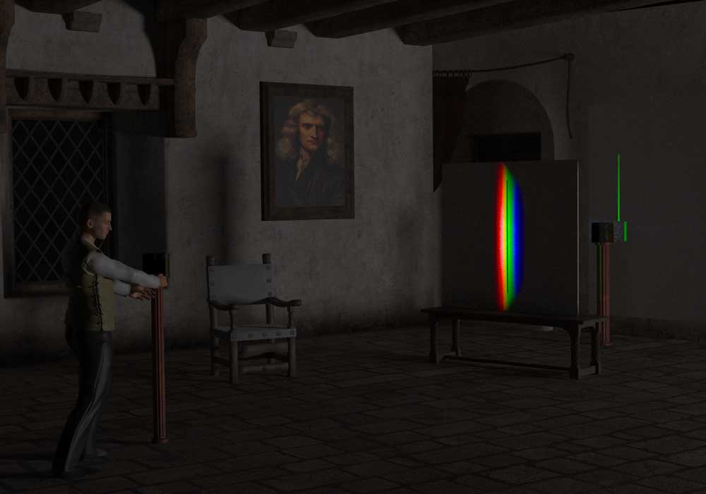
Adding a second prism gives us Isaac Newton’s ‘Experimentum Crucis’: one of a series of experiments performed by Newton in 1666 and reported in a letter to the Royal Society in 1671 (1), showing how white light is composed of a range of colours separable by a prism.
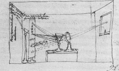
Newton then demonstrated the colours were a property of the light, not the prism, by using a slit to isolate an individual colour from one prism, and passing it through a second where no further separation of colours occurs – the second prism just refracts the single colour to one side. Here is Newton’s own drawing of his two-prism experiment.
Experimentum Crucis
Virtual set-up and approximations
My distances and prism sizes are not accurate, but the simulation still works. Also, Newton used the sun as a light source: passed through a slit before the first prism or focused through a lens. By contrast, my source is a small rectangular surface radiating in all forward directions followed by a collimating tunnel.
If the real or simulated light source is too ill-defined or unfocused, the separation in the spectrum can look superficially reasonable, but actually comprise several fuzzy overlapping spectra. As a result, running without the collimator caused the green band to split into further colours. That said, it’s worth remembering that while Newton reported seeing seven colours, the actual spectrum is a continuum of wavelengths, so a single colour will in fact be made of a range of further dispersible shades – we just don’t discern it.
Results
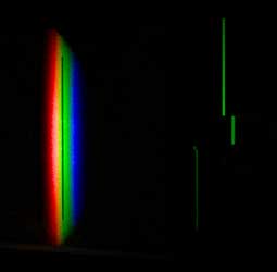
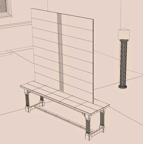
Here is a close-up of the isolating slit and the green spectral ‘line’ deviated but not dispersed by the second prism. I’ve also in this picture turned out the background light used solely for dramatic effect in the first picture.
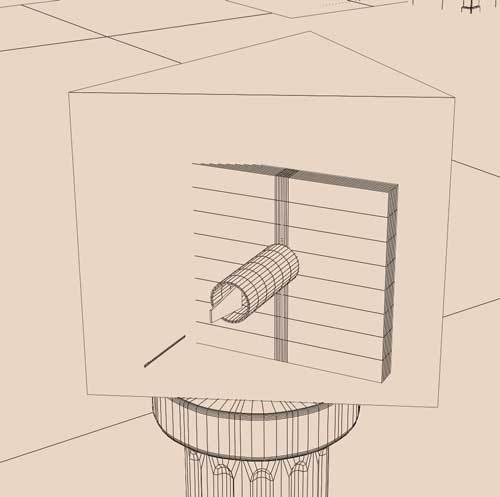
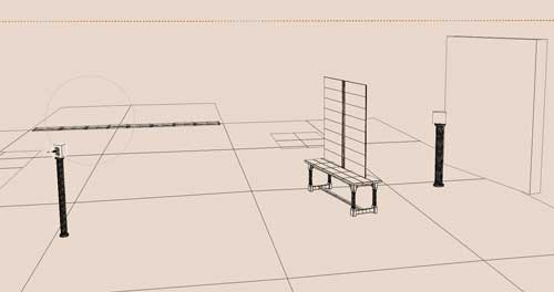
And here are wireframe pics of the layout (scene created in Poser and linked to Luxrender via Reality):
Other Observations
An interesting feature of this type of modelling is the need for a so-called Tone Mapping process. This requires the multiple wavelengths to which the ray-tracing maths is applied to simulate dispersion are translated into the red, blue, and green (RGB) that the computer monitor can display.
This sort of progam is limited as a virtual optical bench. Luxrender cannot, for example, calculate the quantum probability amplitudes necessary to simulate interference as seen in the double slit experiment.
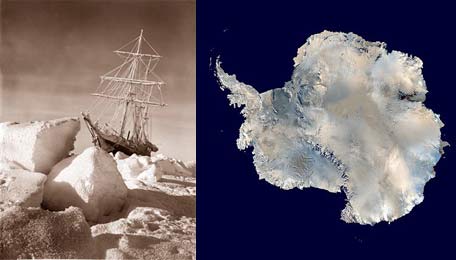
In May 1915, Ernest Shackleton and the crew of Endurance entered their fourth month trapped in the frozen Antarctic’s Weddell Sea. The ship’s navigator added to the gloom forecasting a sunless sky for the next seventy days. You expect this at above 75° South. Then on the 8th of May something strange happened. The Sun reappeared – several times:
The sun, which had made “positively his last appearance” seven days earlier, surprised us by lifting more than half its disk above the horizon on May 8. A glow on the northern horizon resolved itself into the sun at 11 a.m. that day. A quarter of an hour later the unseasonable visitor disappeared again, only to rise again at 11.40 a.m., set at 1 p.m., rise at 1.10 p.m.. and set lingeringly at 1.20 p.m.
Ernest Shackleton, 19151
Shackleton understood the effects of atmospheric refraction, that temperature and density differences can bend light, especially near the horizon. At sunrise and sunset the Sun’s disk may appear lengthened or flattened, or displaced from its true position in the sky.
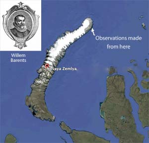
Ernest Shackleton made his observations from the Endurance while frozen in the Weddell Sea (the bay top left)
Mariners knew of the phenomenon, referencing standard refraction tables to correct sextant readings for navigation; but the system broke down below about 6 degrees, where refraction increased rapidly and non-linearly.
In this case, as Shackleton recorded in his journal, the Sun was 2 degrees and 37 minutes (2°37′) from its true position, 2 degrees more than the refraction tables predicted. Plotting position from this observation would place the Endurance 120 miles from its actual location.
The Novaya Zemlya Effect
What Shackleton experienced was an extreme case of atmospheric refraction known as the Novaya Zemlya effect.
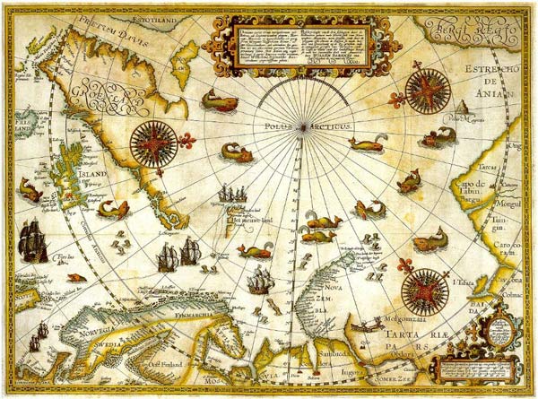
It was first reported in 1597 by Gerrit De Veer2 , one of the crew on Willem Barent’s third voyage to discover a north-east passage. Obliged to hunker down for the polar winter in a safety hut or ‘Het Behouden Huijs‘ built on the Novaya Zemlya island chain north of Russia, De Veer reported the return of the post-winter Sun a whole two weeks before it should have been visible. It was in fact 5°26’ below the horizon. The same thing happened two days later, the Sun still – by the book – 4° below the horizon.
Map depicting Willem Barents three voyages to discover a North East Passage, showing the Novaya Zemlya islands (Wikipedia)
The Novaya Zemlya effect occurs in Arctic regions where tracts of cold air remain uniquely stable over hundreds of kilometers, creating a special instance of a meteorological temperature inversion. The distortion, powerful enough to bend light through four or five degrees, can make celestial bodies like the Sun or Moon appear wholly above the horizon when they are physically below it. (If you imagine looking at the horizon, five degrees is the same as ten Suns or Moons in a row.)
For hundreds of years, nobody believed Gerrit De Veer’s solar observations, and equally his report of a curiously displaced conjunction of the Moon and Jupiter. He must have counted the days wrong, or used the wrong sort of calendar. It took the corroborating reports of polar explorers like Shackleton and, as recently as 2003, ray-tracing simulations3 using contemporary atmospheric data, to fully vindicate De Veer.
I’ve set up my own simulations of the celestial events reported by Shackleton and De Veer using the planetarium software Starry Night. The program can’t reproduce the ray traced refraction effects modeled by van der Werf et al3 – whose validity I’m not equipped to comment on by the way, but it’s still satisfying to check the published numbers and get a feel for what the events looked like all those years ago.
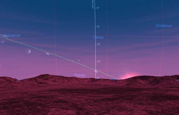
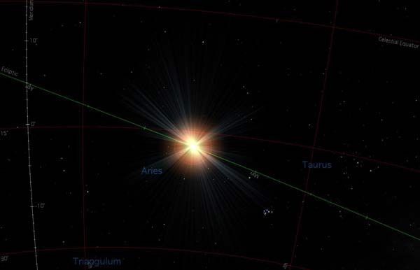
The horizon terrain here is generic Starry Night; apart from being icy-white, the true horizon would run perpendicular to and cross the graduated white Meridian line at zero (0) degrees. The green line is the Ecliptic. Things are clearer for our purposes, if less romantic, if we turn off the daylight effect and fancy terrain and zoom in a bit. It’s now clear the Sun was below the horizon when Shackleton reported seeing it: i.e. with reference to the Meridian on the left, the Sun looks about two and half degrees below the zero degree mark (Shackleton’s 2°37′):
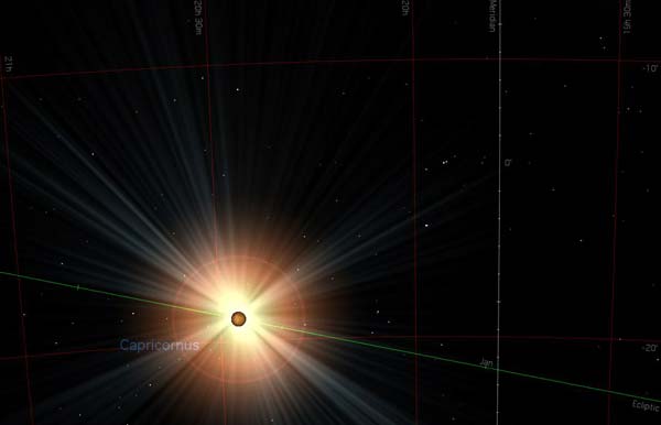
Willem Barent’s crew, marooned 300 years earlier at the opposite end of the planet, made their observations from the ‘Behouden Huijs‘ at coördinates 76° 15.4′ North 68°18.6’ East, Novaya Zemlya. This view from the Huijs at 7 o’clock on the morning of 24th January 1597, shows the Sun was firmly below the horizon when Gerrit De Veer observed it – a whole 5°26′ below (horizon is perpendicular to the zero mark on the white Meridian line, green line is the Ecliptic):
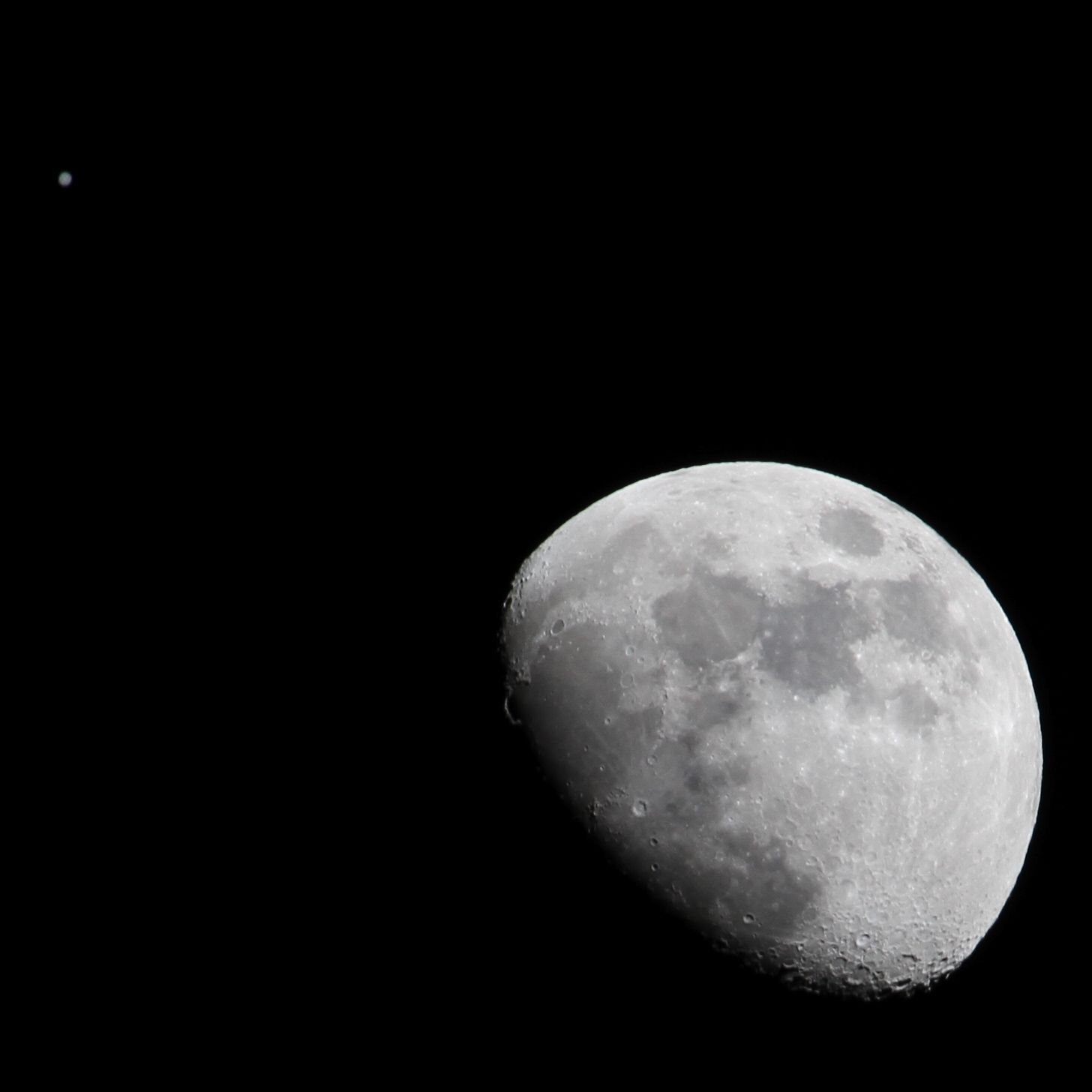
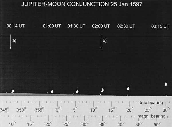
The Moon-Jupiter conjunction reported by De Veer physically happened at 0:14 UT on 25th January 1597 (there is a small error in the 0:24 UT time given in the contemporary tables by Scala that De Veer used). Like astronomers today, De Veer identified the moment of conjunction as the time when a line drawn along the shadow separating light from dark on the moon’s surface, the terminator, pointed directly at Jupiter, as in this photograph I took of the Moon-Jupiter conjunction of 21 January 2012:
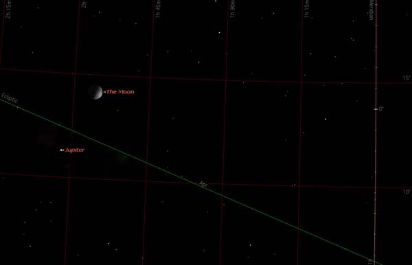
The Moon is barely above the horizon and Jupiter is below it (again, reference the zero on the white Meridian line).
Gerrit De Veer saw this view, but over an hour after it happened: i.e. at 01:27 UT not 00:14 UT. As van der Werf’s analysis explains, De Veer reported the conjunction at 6 a.m. local time, which was 4:33 hours ahead of UT. Such was the unbelievable power of the Novaya Zemlya effect to make this happen that few indeed believed it. De Veer learned about the conjunction from his copy of the Ephemerides of Josephus Scala which gave times for Venice. Here we pick up the story in De Veer’s own words and the spellings of his 1609 translator William Phillip:
Whereupon we sought to knowe when the same coniunction should be ouer or about the house where we then were; and at last we found, yt the 24 day January was the same day whereon the coniunction aforesaid happened in Venice, at one of the clocke in the night [= 1 in the morning of 25th Jan], and with vs in the morning when ye sun was in the east: for we saw manifestly that the two planets aforesaid approached neere vnto each other, vntill such time as the moone and Jupiter stood ouer the other, both in the sign of Taurus, and that was at six of the clocke in the morning;at which time the moone and Jupiter were found by our compas to be in coniunction, ouer our house..
Gerrit De Veer 1597
Yet ray tracing the scenario 400 years later, with Jupiter two degrees below the horizon and the Moon just above it at conjunction, shows that atmospheric conditions raised Jupiter’s apparent position disproportionately to that of the Moon. Moreover, the simulation reproduced what De Veer saw at the time he saw it: a conjunction visible to him at around 02:00 UT. The ray tracing team made a further minor adjustment for the Equation of Time effect, which brought their estimate of when the conjunction was visible to De Veer as 06:20 local time, which is impressively close to his 06:00.)
Apparent position of Jupiter and the Moon after allowing for atmospheric refraction. Moon is double actual size for clarity. Diagram reproduced from analysis by van der Werf et al, 2003 (reference 3)
One More Thing
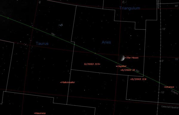
Although Gerrit De Veer’s vindication now seems complete, there was one little alarm bell went off during my research, concerning De Veer’s reference to both the Moon and Jupiter being in the constellation of Taurus at the time of conjunction. Zooming in to see the 1597 conjunction against modern constellation boundaries puts it well into Aries. So what gives?
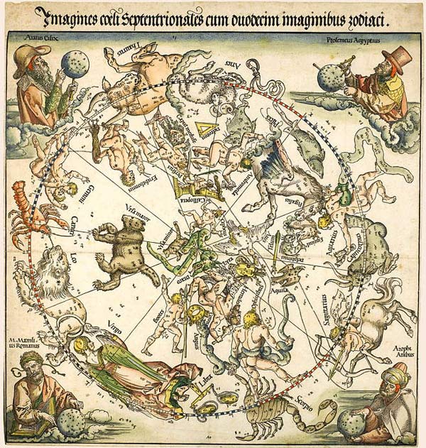
Maybe the constellation boundaries have changed; let’s have a look at Albrecht Dürer’s beautiful star chart from 1515. Here we see the belly of the bull tucks a little further under the ram than in modern charts, but the conjunction is still firmly in Aries.
Star chart of the northern skies, Albrecht Dürer, 1515, Nuremberg.
Maybe the Moon made the stars in Aries harder to see that night. That might cause De Veer to focus on the sparkling Pleiades and Hyades clusters in Taurus. (I’d probably do that if I were standing in a freezing Arctic wasteland staring at the sky at six in the morning.)
Charles Beke4 also noticed the discrepancy in a 19th century analysis of the William Phillip translation. He points to a retrogression of the equinoctial points – the places where the celestial equator intersects the ecliptic. Since De Veer’s day, this will have shifted the positions of the constellations in terms of longitude and latitude relative to those references. Although that suggests De Verre placed the conjunction in whatever constellation the numbers dictated, rather than where he saw it? Still a bit of a mystery to solve then – at least in my mind.
References
E. Shackleton, South: The Story of Shackleton’s Last Expedition 1914–1917, MacMillan, New York, 1920
Gerrit De Veer, The Three Voyages of William Barents to the Arctic Regions (1594, 1595 and 1596). London, 1876 (translation of 1609 original).
Charles T. Beke, The Three Voyages of Willem Barents to the Arctic Regions 1594, 1595 and 1596 by Gerrit de Veer, 2nd ed.William Phillip, trans., Hakluyt Society, London, 1876 (Page 147)
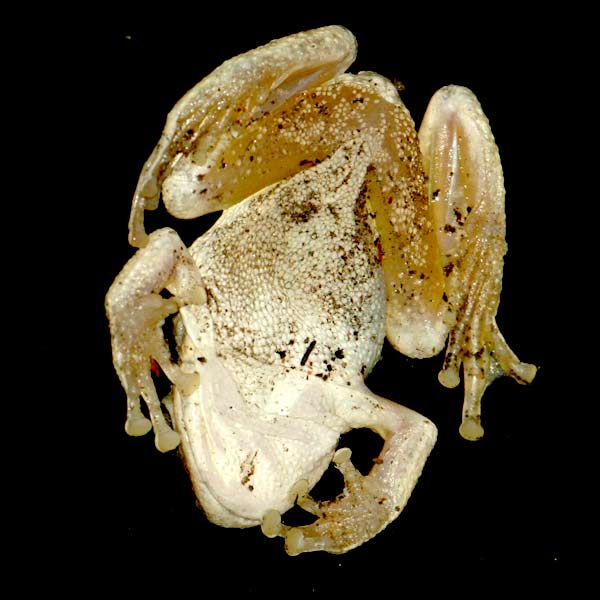
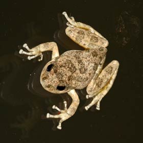
Tree frogs in trees are just fine, but tree frogs on plate-glass windows are better – because then you get to see their slightly icky fascinating undersides.
I must admit, what struck me most when this guy landed – ‘thunk’ – out of a fig tree onto our window in Los Angeles, was how much his (her?) legs looked like raw chicken. I’ve always shied away from those cuisses de grenouille opportunities, but I know the meat is often compared to chicken. Why frogs and chickens developed that way is an interesting question, but not for today’s post.
Rather, now I’m back in the UK , where the frogs are less acrobatic, I’ve tried to figure out how our unexpected visitor managed to cling on.
Wet Adhesion
To understand that for the West Indian tree frog, Oseopilus septentrionalis, researchers Hanna and Barnes1 used active and anaesthetised frogs in experiments that measured the forces they apply walking up vertical surfaces, the angle at which they drop off a gradually inclined surface, and the shear force experienced by an individual toe when the surface it’s attached to is suddenly slid from under it.
The experiments involved placing frogs on a variety of strain-gauge instrumented platforms and surfaces, and making videos of frogs placed on runways and rotating discs of transparent perspex.
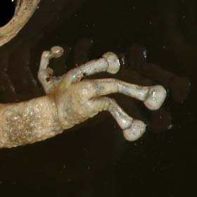
The researchers concluded that the primary mechanism tree frogs use to get a grip is exactly the same as that which keeps a sheet of wet paper stuck to the side of a glass: wet adhesion.
Wet adhesion combines a mix of viscous and surface tension forces, both of which require liquid and, in the case of surface tension, an air-liquid interface. In the tree frog, that liquid takes the form of mucous – wait for it – pumped out the ends of its toes.
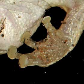
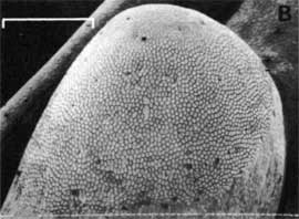
The mucous appears from perfectly smooth-looking toe pads that are actually covered in thousands of peg-like cells between which mucous flows from glands. I can see something going on in my own photographs, but the structure is clear in the SEM picture below.
Hanna and Barnes’s also looked at how tree frogs release themselves to move. The frogs peeled rather than pulled their feet off surfaces, the peeling force engaging automatically in forward movement, but not in reverse or when the belly skin of the frog made contact with the surface.
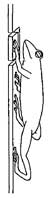
Frogs placed on a slowly rotating vertical disc reorientated themselves to avoid facing downwards – presumably because of the involuntary forward travel or detachment that would induce. At first sight then, my Pseudacris cadaverina appears to defy that rule – because he’s clearly inverted in one of the pictures; but that could be explained by the extra adhesion he’s getting from the inner thigh area – corresponding to the aforementioned belly skin. What’s more, the authors point out that toe pads have developed independently several times in tree frogs, so the observed peeling mechanism may be peculiar to Oseopilus septentrionalis.
I would have liked to spend more time with this little guy, but after about ten minutes I looked up and he’d gone – probably back into the fig tree. But for a while there he sure provided a level of interest, conversation, and intrigue way out of proportion to his size. Ribbit.
Apparatus to measure climbing force
Tree frog toe pad. After Hanna & Barnes, 1991.
References
1. Adhesion and detachment of the toe pads of tree frogs. Gavin Hanna, W.John Barnes. Journal of Experimental Biology 155, 103-125 (1991)
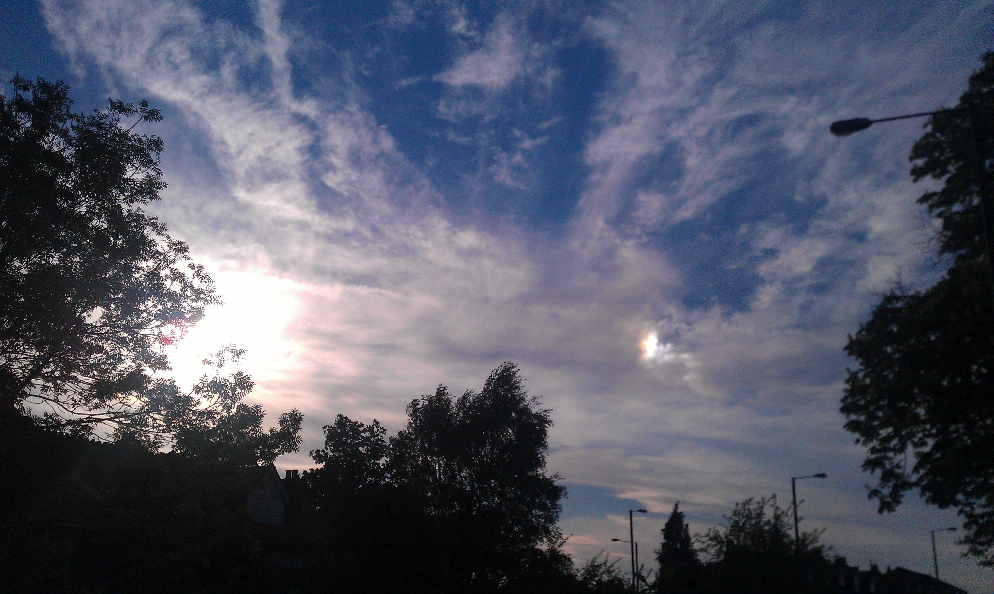
A Sun Dog in Surrey. Sun is on the left, the sun dog is the patch of light to the right (Photo:Tim Jones)
Despite keeping an eye out for strange atmospheric phenomena, my track record is not good, and I count myself lucky to catch the occasional rainbow. Lots of sailing, flying, and mountain walking over the years, with nice low, clear, horizons, and I’ve yet to see the almost mythical ‘Green Flash’.
But yesterday I saw a special type of mini-rainbow: a Sun Dog.
The concentrated patches or spots of light can be very bright, always at the same level of the sun, and always at a 22 degree angle from the sun.
They’re caused by light passing through clouds of ice crystals in the upper atmosphere, typically above 10 km. Ice crystals are all hexagonal in cross-section, and vary in size and length; but under the conditions that generate a sun dog, the crystals have become aligned in the air flow (because they’ll have a minimum air resistance in a shared direction) so that light passing through them leaves in the same direction: hence the 22 degrees.
I’ve seen photos of sun dogs, and may have seen fainter patches of rainbow that were actually unconvincing sun dogs. But this one was really bright, like a little sun hanging where it shouldn’t be. You’ll know it if you see one.
And if that’s piqued your interest for atmospheric phenomena, here’s an excellent lecture from Professor of Astronomy at Gresham College, Carolin Crawford, who explains better than I can Sun Dogs (from around 44 mins) and a whole bunch of other effects that I never knew existed.
After watching this lecture again, I think there’s also a bit of Coronae interference scattering visible in my photo: that pink/purple glow near the sun.
Historic olla water cooling pots made by Native Americans in San Diego County. Possibly Kumeyaay or Diegueno origin. (Photo:Tim Jones)
Maybe it was the furnace heat of California last month, or the topicality of NASA’s Curiosity landing, but here I am having my first – and almost certainly last – von Däniken moment.
Olla
Mars
How else though, aside from some ancient Martian visitation, could Native Americans of centuries past, without the benefit of telescopes or interplanetary probes, design water pots so closely matching the Red Planet?
Well, on reflection, I guess a mixture of clay and cactus juice might just bake out that way in the sun.
Which brings us to the real science behind these earthenware pots. Because although they may well be over two hundred years old, discovered in 1926 by my wife’s geologist great-grandfather in the desert of San Diego County, these water carrying olla represent nothing less than the world’s first refrigerator.
The larger olla in-situ, San Diego County, 1926, complete with geological hammer for scale. Ollas were not truly ‘fired’, but hardened by baking in the sun (Scan of original photo belonging to Tim Jones)
The water inside the olla reaches a temperature substantially below that of the surroundings thanks to the principle of evaporative cooling – something you can demonstrate to yourself just by licking a finger and waving it around. The skin feels cooler because the heat needed to turn liquid water molecules in your spit into vapourised water molecules leaving your hand is taken from your skin. The amount of heat, or energy, needed to change from a liquid to a gas is called the latent heat of evaporation, which for water is 2257 kJoules per kilogram.
Kumeyaay (Wikipedia)
The sun-baked porous clay of the olla acts like a wick, delivering a constant flow of evaporating water to the surface where it quickly evaporates, cooling first the surface and in turn the water inside the pot.
Wondering how effective ollas really are, but with live tests on our delicate pots off the agenda, I turned to theoretical musings and some (not entirely successful) experimentation.
The Theory
The temperature on the pot’s surface, or wet-bulb temperature, is easy enough to calculate if we know the ambient air temperature, relative humidity (how much water is already in it), and local air pressure – as that affects the dew-point temperature at which water changes from liquid to gas. I got all that info from my local weather station online, and plugged it into one of the many online calculators – like this one at the National Oceanic and Atmospheric Administration (NOAA) – to find the wet bulb temperature. (The exact calculation is complex and explained on the NOAA website, but essentially the drier the air, the lower the wet-bulb temperature; water molecules already in the air decrease the net evaporation rate.)
The day I looked at this, the values were: temperature 34 C, relative humidity 20%, and air pressure 1014.9 millibars, for which the NOAA calculator returned a wet-bulb temperature of about 19 C. That’s a whole 15 degrees below ambient temperature; modern electric fridges don’t do much better than that (okay – granted they can get to lower absolute temperatures).
Wet-bulb thermometer (Photo:Tim Jones)
The wet-bulb temperature I verified experimentally using a cooking thermometer modified with wet paper-towel stuffed in around the sensor tip (a mercury thermometer would have a bulb of mercury at the end – hence wet-bulb; but this was all I had and works well enough). Swinging the thing fast round my head on the end of a shoelace simulated wind and, lo and behold, I recorded a wet-bulb temperature of 21C. Not quite the predicted 19C, but in the right area.
Good ventilation of the olla is necessary as it influences the evaporation rate, and the area for evaporation should be large (the olla’s spherical design is fantastic in this regard as it maximises the area). The area of non-wetted contact should be small to minimise absorption of heat by conduction from the surroundings – here again, the point contact of the spherical olla is perfect. Ollas also work better in the shade, to minimise heating by solar radiation.
Calculating how long the contents take to cool is more tricky, requiring an estimate of the evaporation rate from a porous surface. But we can get some handle on it using an assumed rate of 7kg/m2.day (based on some data I found for swimming pool evaporation rates in Australia of all things), latent heat of evaporation of water 2257 kJ/kg, and heat capacity of water 4.18 kJ/kg.K. From which I reckon the 0.3m diameter olla, holding 14 litres (=14 kg) of water, needs to lose 878 kJ of heat to fall in temperature by 15 degrees, equal to evaporating 0.4 litres (0.4kg or 3% of the contents) from the 0.28 m2 surface over a 5 hour period.
The numbers aren’t perfect, but suggest in its heyday our olla was up and usefully cooling in a couple of hours.
The Practise
Now for the not-totally-successful experimentation part of the post.
Plant pot evaporative cooler (Photo:Tim Jones)
You can see what I’m trying to do here: my very own plant pot olla. The physical conditions (temp.,humidity,pressure) were the same as the theoretical calculation; and I’d confirmed a wet-bulb temperature of 22C as described above. The pot was kind of working too; that dark band in the middle and top is water seeping through the porous terracotta – and it was pretty consistent throughout the experiment.
Stirring the contents and taking regular measurements indicated a one degree fall over the first two hours. But then the temperature started to climb again, which suggests the pot was just not porous enough over sufficient area to counter heating by conduction through the non-wetted areas. A lack of wind won’t have helped – maybe use a fan next time. At least no one can accuse me of selectively publishing only positive results.
Other Coolers
The Arab Zeer works in a similar fashion to the olla, but consists of two pots separated by wet sand. Fruit and other perishables can be kept fresh in the central pot.
Pot-in-pot, Zeer type evaporative coolers (Wikipedia)
A modern invention is this Terracooler: an evaporatively cooled terracotta bell-jar placed over food to keep it fresh.
Evaporative cooling in water features is enhanced by an electric pump (Photo:Tim Jones)
And keep an eye out for artificial waterfalls used to create a cool atmosphere in public spaces, or the same principle operating in simple garden water features: the water in this one I measured at 24C on a 32C day.
I’m back in the UK now, where typical humidity levels close to 100% (=rain) preclude the extensive program of further evaporative cooling tests this discussion clearly signposts. If you have more luck with your own ollas though, do let me know.
It’s that candlelit dinner stage of the evening. Soup through nuts, you’ve been your wonderful, genuine, self. And he/she is pretty fantastic too.
Spectrum of candle flame by diffraction in a CD (Photo:Tim Jones)
But why take chances – this is deal clinching time.
With the table cleared, quick as a whippet you pull out your Ethereal Collapse CD, and with a flourish Newton would die for if he wasn’t already dead, guide your beloved’s eye to the spectacular demonstration of spectra by diffraction.
Your friend will by now be in a frenzy of excitement, so this is the moment to push them over the edge.
Rushing through to the restaurant kitchen with a mix of urgency and discord normally reserved for Bond movies, you thrust your CD into the light once again. But now the disc reflects the chef’s fluorescent tube in an almost unbearably different, and extremely interesting way. The smooth continuum of the candle flame is gone! Now superposition bands stand proud, where line discharge spectra from gaseous mercury inside the lamp combine with the continuous spectra emitted from the phosphor coating.
Spectrum of fluorescent lamp by diffraction in a CD (Photo: Tim Jones)
At this point, you’ll almost certainly be offered complimentary Cognacs – if only to leave the kitchen. But by now you’ll both be itching to get off anyway, back to his/her flat to repeat the experiments under controlled conditions. Or maybe play some Scrabble.
The Kindle’s supremely convenient, and the iPad’s drop-dead gorgeous. So why do I find Clifford Pickover’s good ol’ fashioned hardback version of The Physics Bookso damn attractive. And I do mean physically – so to speak. (It’s on iPad too, but read on.)
Maybe I’m getting all bookish-protective in the month that Encyclopedia Britannica wound up its iconic print edition after 244 years? Or is the tactile slabbiness of The Physics Book a nostalgic reminder of the Purnell’s and Marshall Cavendish encyclopedias of my formative years? Well, it’s the latter of course; I almost feel like jumping into short trousers for a re-read.
But enough of my fetishes already.
The Physics Book isn’t really an encyclopedia, but the word kind of fits given the breadth of topics covered. For each of 250 Milestones in the History of Physics, we’re given enough information to be useful in its own right, but with signposting for further research; it’s a kind of physics taster if you like. And while I’m sure it’s readable in two or three good sessions, I found myself dipping in and returning over a period of weeks. So much for prompt reviews then, but this is an eminently dipinable book.
When I reviewed Tweeting the Universe, I was impressed how the authors tackled the unassuming little task of explaining the whole universe in a series of 140 word ‘tweets’. Pickover’s offering is a different animal with much more meat on it, but he’s still had to work, effectively I think, at getting a coherent story for each item into one page of text and an accompanying photograph. Also, Tweeting the Universe doesn’t weigh 1.5kg!
Appropriately kicking off with the Big Bang 13.7 billion years ago, the chronological journey is otherwise unsegmented. How could it be? Discoveries don’t just pop up in categories to order. But that also means practical, down-to-earth, physics applications – like the engineering truss – can mingle with less tangible concepts like Pauli’s exclusion principle. And while there’s no talking down to the reader – there are even a few equations! – I think the spattering of examples linking underlying physics to everyday objects and experiences keeps us all onboard.
The engineering references in particular show how some devices we think of as modern were discovered and applied ages ago, even if they weren’t at the time properly understood in a scientific sense; it turns out the first electric battery pre-dated Volta by a whole millenium. In other news, we’ve only recently come to grips with why ice is so slippery – and it might not be why you think. We only figured out how the hourglass works in a 1996 physical modelling study at the University of Leicester (as it happens the city I originally hail from and an area of research technique I used to work in). Other apparently simple observations still lack a satisfactory explanation, like the mysterious black drop effect that happens when Venus transits the sun.
A repeating theme is discoveries being made independently by more than one person, like the explanation of rainbows, calculus, and the laws of refraction: a reminder perhaps that we discover scientific knowledge, not make it up depending on who we are, where we are, or which culture we belong to. There are also lessons in the less than intuitive nature of some relationships, like that between fluid volume and pipe size (Poiseuille’s Law).
The popular association of physics with weapons – typically represented by the iconic atom bomb mushroom cloud – is not neglected or shied away from. Indeed, Pickover describes a range of weapons enabled by physics through the centuries. I knew about the boomerang and crossbow, but the prehistoric atlatl technology, exploiting the principle of leverage to kill mammoths and conquistadors with indiscriminating effectiveness, was news to me.
Pickover’s references are diverse, with lots of modern day and ancient quotations from commentators ranging from Aristotle to Einstein, references to fiction and science fiction, and some pan-cultural associations you wouldn’t expect. Who knew Edgar Allen Poe first suggested a solution to Olber’s Paradox “Why is the sky dark at night?”.
Certain pre-eminent individuals like Newton, Einstein, and Hawking, as sources of particular inspiration, get their own pages. William Gilbert De Magnete gets a mention as the first guy to break god’s monopoly on knowledge and start doing proper experiments, as does Eratosthenes for the shear elegance of his Earth circumference calculation from observation and deduction. Talking of experiments, it’s not the main idea, but there are a few prompts to try stuff at home, like breaking candy bars or pulling off lengths of scotch tape in the dark to see the triboluminescence.
If big picture, left-field, even spooky physics are your thing, ideas like Quantum Mechanics (including Quantum Electro-dynamics) and Heisenberg’s Uncertainty principle are generously discussed; also my favourites: Spooky Action at a Distance (Quantum Entanglement, Bell’s Theorem), and stellar nucleosynthesis. It’s a reminder we’re all made of star stuff, and that reality is weird enough without us making up any extra fairy stories. Other entries in this vein border on the philosophical (another discipline gobbled up by physics?), like the totally plausible if challenging thought that we might all be living in a Matrix-style simulation. Then there is Quantum Immortality – the idea that across infinite multiple universes we might live effectively, necessarily, forever. Likelihood is after that lot you’ll only be good for browsing the photos.
So just as well there are lots of them – precisely 50 percent by page area. My favourite – I think I go for shots with people in them – shows observatory staff posing somewhat precariously on the mount of the University of Pittsburgh’s Thaw refracting telescope. I also like the shot of Stanley and Lawrence standing by their cyclotron. Other pictures illustrate applications – good and bad: like the squat ‘Little Boy’ atomic bomb sitting innocently in its cradle: a simple photograph that evokes so many complex thoughts. Or more constructively, a Nuclear Magnetic Resonance (NMR) picture of arteries in the head, for me the ultimate expression of applied, useful, physics. Some pictures are just fun – like Schrodinger’s Cat peeping out of a cardboard box with a “what?” expression on its face.
Moreover, we’re left in no doubt that physics gets everywhere. It’s a bit of a joke across the scientific disciplines, in a sour-grapes sort of way, that all the other sciences are a subset of physics. That’s not the case, but Pickover’s examples for sure underscore physics’ broad reach. I love the way diffusion and Brownian Motion explains the spread of muskrat populations.
So there you go. My impressions and a bit of a content summary of items that stuck with me from The Physics Book. There’s nothing not to like, and despite my reminiscences from childhood, I’m sure readers of all ages and backgrounds will enjoy it – in iPad or ‘real book’ form!
“The truth is stranger than fiction” (Mark Twain and Todd Rundgren)
Richard Feynman’s Grave at Mountain View Cemetery (Photo:Tim Jones)
Today I paid my respects at the grave of physicist Richard Feynman, interred with his wife Gweneth at the Mountain View Cemetery in Altadena, California. Feynman died of cancer in 1988 and his wife died the following year.
The grave is marked by a very simple plaque, which my wife and I would never have found without the help of the cemetery staff. Even then, until we brushed it off, the plaque was barely visible among the leaves and twigs – fallout from the Santa ana winds that have just ripped through the region.
Richard Feynman at Fermilab. Image in public domain and available via Wikicommons
Today was calm and sunny though, and the cemetery is a beautiful spot to find yourself. Lots of trees with birds and squirrels running about, the whole overlooked by the San Gabriel Mountains and Mount Wilson (of 100 inch telescope fame).
Feynman researched and taught as Professor of Physics at the nearby California Institute of Technology in Pasadena from 1950 until his death.
Here are some more photos at the cemetery:
If you don’t know about Richard Feynman, I recommend in addition to his Wikipedia page you check out the biographies Genius by James Gleick, and Quantum Man by Lawrence Krauss. I also enjoy failing to completely understand (note the word order) Feynman’s 1979 Douglas Robb Memorial Lectures on Quantum Electro-dynamics (QED).
More recently, here’s physicist Leonard Susskind’s personal insight on the man in his January 2011 TED talk ‘My friend Richard Feynman’
Lunar Eclipse, 10th December 2011, 5.40 PST from Los Angeles (Photo:Tim Jones)
I took these photographs between 5.00 and 6.15 a.m., 10th December 2011, from the foothills above Los Angeles near Pasadena. Here’s the progression through to totality at around 6.05 a.m.
Pics taken on Canon 7D, 100-400 L, Various ISO 200-800, 100th" - 1" f6.3
Lunar Eclipse, 10 Dec. 2011, 5.15 PST, Los Angeles, Photo:Tim Jones
Lunar Eclipse, 10 Dec. 2011, 5.24 PST, Los Angeles, Photo:Tim Jones
Lunar Eclipse, 10 Dec. 2011, 5.33 PST, Los Angeles, Photo:Tim Jones
Lunar Eclipse, 10 Dec. 2011, 5.35 PST, Los Angeles, Photo:Tim Jones
Lunar Eclipse, 10 Dec. 2011, 5.39 PST, Los Angeles, Photo:Tim Jones
Lunar Eclipse, 10 Dec. 2011, 5.40 PST, Los Angeles, Photo:Tim Jones
Lunar Eclipse, 10 Dec. 2011, 5.50 PST, Los Angeles, Photo:Tim Jones
Lunar Eclipse, 10 Dec. 2011, 5.50 PST, Los Angeles, Photo:Tim Jones
Lunar Eclipse, 10th Dec 2011, 5.55 PST, Los Angeles (Photo:Tim Jones)
Lunar Eclipse, 10th Dec 2011, 6.00 PST, Los Angeles (Photo:Tim Jones)
Lunar Eclipse, 10th Dec 2011, 6.02 PST, Los Angeles (Photo:Tim Jones)
Lunar Eclipse, 10th Dec 2011, 6.04 PST, Los Angeles (Photo:Tim Jones)
Lunar Eclipse, 10th Dec 2011, 6.04 PST, Los Angeles (Photo:Tim Jones)
Lunar Eclipse, 10th Dec 2011, 6.08 PST, Los Angeles (Photo:Tim Jones)
Lunar Eclipse, 10th Dec 2011, 6.11 PST, Los Angeles (Photo:Tim Jones)
Lunar Eclipse, 10th Dec 2011, 6.11 PST, Los Angeles (Photo:Tim Jones)
I’d heard of Alain de Botton’s School of Life and its “good ideas for everyday living“; I just hadn’t been to one of their ‘Sunday Sermons’.
Krauss 2.0 ?
So arriving at Conway Hall yesterday to hear theoretical physicist and all-round science communicator Professor Lawrence Krauss talk about Cosmic Connections, it was an unexpected but not disagreeable surprise to find David Bowie and a seven foot spandex-clad devil stirred into the mix. I for one can’t think of a better preparation for contemplating one’s insignificance in a miserable futureless universe than a good singalong to Space Oddity.
Conway Hall (Photo:Tim Jones)
“You are stardust; it is literally the most poetic thing I know about in all of science”
On the face of it, Krauss’s ultimate message is a bit grim: that our expanding, accelerating, universe will eventually dilate into cold, empty, blackness. But, more positively, he’s saying we should take all that as read and concentrate on our perspective: understand what we really are and how we connect with the universe. Then the journey to oblivion doesn’t look so miserable afterall; it looks fascinating – even poetic.
Stardust meets Starman
Krauss’s consciousness-raising / cheer-up therapy centred around three less than obvious connections we have with the cosmos:
First off – we are the universe. We’re made of stars. The heavy elements that make us up could only have been made in stars, and they could only end up as part of us if they were blasted out of exploding stars: the supernovae.
You were here…
Call me a romantic, but I like the imagery. Bits of me: hands and feet, arms, legs, head, brain – they didn’t just pop up a few decades ago, but have been flying around for billions of years and will be around for billions more. I’ve been inside an exploding supernova – several most likely.
Straight on at purgatory, then right at the second circle….
What the….
Next came the connectedness of life, with a nice story of Krauss sitting to write a physics paper, aware he’s breathing the very atoms breathed by Einstein as he formulated his own theories (inspired inhalation?). We’ve all got a bit of Julius Caesar in us it seems – literally. And on the larger scale of the solar system, the exchange of possible life-bearing rocks between the Earth and other planets, including Mars, could mean we’re all extra-terrestrials without even knowing it.
“The future is miserable”
Krauss’s final illustration challenges our perception that aspects of reality we normally consider outlandish and irrelevant to our day-to-day life do indeed have a direct influence on us. The mundane activity in question is navigation by Global Positioning System (GPS), where the consquences of not correcting for satellite speed (Special Relativity), and height above the Earth (gravity effect/General Relativity), on measurement of the requisite nano-second scale signal transit times, would in only a day be sufficient to put ground track navigation out by several kilometres.
“Ground control to Major Tom”
“Bits of Mars are falling on Earth all the time”
I really like this GPS example and the way Krauss presented it. There was no such thing as GPS when I was at school, so all we got were stories of atomic clocks losing time when they were shot round the world on fast planes, or hypothetical astronauts of the future going on fictional journeys. To be able to relate relativistic effects to a very real navigational error that normal folk can recognise and care about is brilliant.
Who’d have thought Sunday sermons could be such fun?
This website uses cookies to improve your experience while you navigate through the website. Out of these, the cookies that are categorized as necessary are stored on your browser as they are essential for the working of basic functionalities of the website. We also use third-party cookies that help us analyze and understand how you use this website. These cookies will be stored in your browser only with your consent. You also have the option to opt-out of these cookies. But opting out of some of these cookies may affect your browsing experience.
Necessary cookies are absolutely essential for the website to function properly. This category only includes cookies that ensures basic functionalities and security features of the website. These cookies do not store any personal information.
Any cookies that may not be particularly necessary for the website to function and is used specifically to collect user personal data via analytics, ads, other embedded contents are termed as non-necessary cookies. It is mandatory to procure user consent prior to running these cookies on your website.

")


")
")

")
")
")
")
")
")
")
")


")


")
")
")
")
")
")
")
")

")


